Godines et al. 2025
Figure 1 - Disk Model
The following code shows how we set up our disk model using the disk_model module. This model was used to configure the simulations, including the calculation of the stokes numbers, pressure gradient parameter and strength of the self-gravity at the three different disk locations. Note that the Model class object containts the get_params method which prints the calculated disk parameters.
import numpy as  np
import matplotlib.pyplot as plt
import astropy.constants as const
from protoRT import disk_model

try:
    import scienceplots
    plt.style.use('science')
    plt.rcParams.update({'font.size': 26,})
    plt.rcParams.update({'lines.linewidth': 1.5})
except:
    print('WARNING: Could not import scienceplots, please install via pip for proper figure formatting.')
    plt.style.use('default')

# Mass of the star
M_star = const.M_sun.cgs.value

# Mass of the protoplanetary disk
M_disk = 0.02*const.M_sun.cgs.value

# Radii which to model, and the characteristic radius of the disk (in [au])
r, r_c = np.arange(5,110.25,0.25), 300

# Convert to cgs units
r, r_c = r*const.au.cgs.value, r_c*const.au.cgs.value


## Disk model adopted in this work (Section 2.1 of the paper) ##
## Used to convert our multi-species simulations with self-gravity from code units to physical units (cgs) ###

# Internal dust grain density (from DSHARP dust model)
grain_rho = 1.675

# Dust to gas ratio (Equation 11)
Z = 0.03

# Temperature power law index (Equation 2)
q = 3/7.

# Temperature at r = 1 au (Equation 2)
T0 = 150

# The sizes of the four dust grains in our simulations
grain_sizes = np.array([1.194, 0.3582, 0.1194, 0.03582])

# The Model class in the disk_model module only works with one grain size, so we define four unique models
# All other model parameteres are the same so these models only differ in their respective Stokes number
model_2a = disk_model.Model(r, r_c, M_star, M_disk, grain_rho=grain_rho, grain_size=grain_sizes[0], Z=Z, stoke=None, q=q, T0=T0)
model_2b = disk_model.Model(r, r_c, M_star, M_disk, grain_rho=grain_rho, grain_size=grain_sizes[1], Z=Z, stoke=None, q=q, T0=T0)
model_2c = disk_model.Model(r, r_c, M_star, M_disk, grain_rho=grain_rho, grain_size=grain_sizes[2], Z=Z, stoke=None, q=q, T0=T0)
model_2d = disk_model.Model(r, r_c, M_star, M_disk, grain_rho=grain_rho, grain_size=grain_sizes[3], Z=Z, stoke=None, q=q, T0=T0)

# Plot
fig, axes = plt.subplots(nrows=5, ncols=1, figsize=(8, 20), sharex=True)
fig.subplots_adjust(hspace=0.075)

# Plot 1: Surface Density
axes[0].plot(model_2a.r / const.au.cgs.value, model_2a.sigma_g, c='k', linestyle='-', label='Gas')
axes[0].plot(model_2a.r / const.au.cgs.value, model_2a.sigma_d, c='k', linestyle='--', label='Dust')
axes[0].set_ylabel(r'$\Sigma$ (g cm$^{-2}$)')
axes[0].set_yscale('log')
axes[0].legend(frameon=False, loc='upper right', handlelength=0.75)
axes[0].set_title('Protoplanetary Disk Model')

# Plot 2: Temperature
axes[1].plot(model_2a.r / const.au.cgs.value, model_2a.T, c='k', linestyle='-')
axes[1].set_ylabel(r'T (K)')
axes[1].set_ylim((20,80))

# Plot 3: Stokes Number
axes[2].plot(model_2a.r / const.au.cgs.value, model_2a.stoke, c='k', linestyle='-', label='12 mm')
axes[2].plot(model_2c.r / const.au.cgs.value, model_2c.stoke, c='k', linestyle='--', label='1.2 mm')
axes[2].plot(model_2b.r / const.au.cgs.value, model_2b.stoke, c='k', linestyle=':', label='3.6 mm')
axes[2].plot(model_2d.r / const.au.cgs.value, model_2d.stoke, c='k', linestyle='-.', label='0.36 mm')
axes[2].set_ylabel('St'); axes[2].set_yscale('log')
axes[2].set_ylim((0.001, 5.25))

# Add vertical lines
axes[2].axvline(x=10, linestyle=':', linewidth=2.5, color='red', alpha=0.65)
axes[2].axvline(x=30, linestyle=':', linewidth=2.5, color='red', alpha=0.65)
axes[2].axvline(x=100, linestyle=':', linewidth=2.5, color='red', alpha=0.65)
legend = axes[2].legend(loc='lower right', handlelength=0.75, ncol=2)

# Plot 4: Scale Height
axes[3].plot(model_2a.r / const.au.cgs.value, model_2a.h, c='k', linestyle='-')
axes[3].set_ylabel(r'H/r')
axes[3].set_ylim((0.04, 0.1))

# Plot 5: Toomre Q Parameter
axes[4].plot(model_2a.r / const.au.cgs.value, model_2a.Q, c='k', linestyle='-')
axes[4].set_ylabel(r'$Q$'); axes[4].set_xlabel('Radius (au)')

# X-axis formatting (hiding x-tick labels for all but the bottom plot)
for ax in axes:
    ax.set_xlim(5., 102.)
    ax.label_outer()

# Add the vertical red dashed lines to denote location of our three simulations
for i in range(5):
    axes[i].axvline(x=10, linestyle=':', linewidth=2.5, color='red', alpha=0.65)
    axes[i].axvline(x=30, linestyle=':', linewidth=2.5, color='red', alpha=0.65)
    axes[i].axvline(x=100, linestyle=':', linewidth=2.5, color='red', alpha=0.65)

# Add vertical text labels aligned with the lines (only lower plot)
axes[4].text(10., 114.037, '10 au', color='red', rotation=90, verticalalignment='top', horizontalalignment='right')
axes[4].text(30., 114.037, '30 au', color='red', rotation=90, verticalalignment='top', horizontalalignment='right')
axes[4].text(100., 114.037, '100 au', color='red', rotation=90, verticalalignment='top', horizontalalignment='right')

# Save
plt.savefig('Disk_Model_SelfGravity_OneColumn.png', dpi=300, bbox_inches='tight')
plt.show()
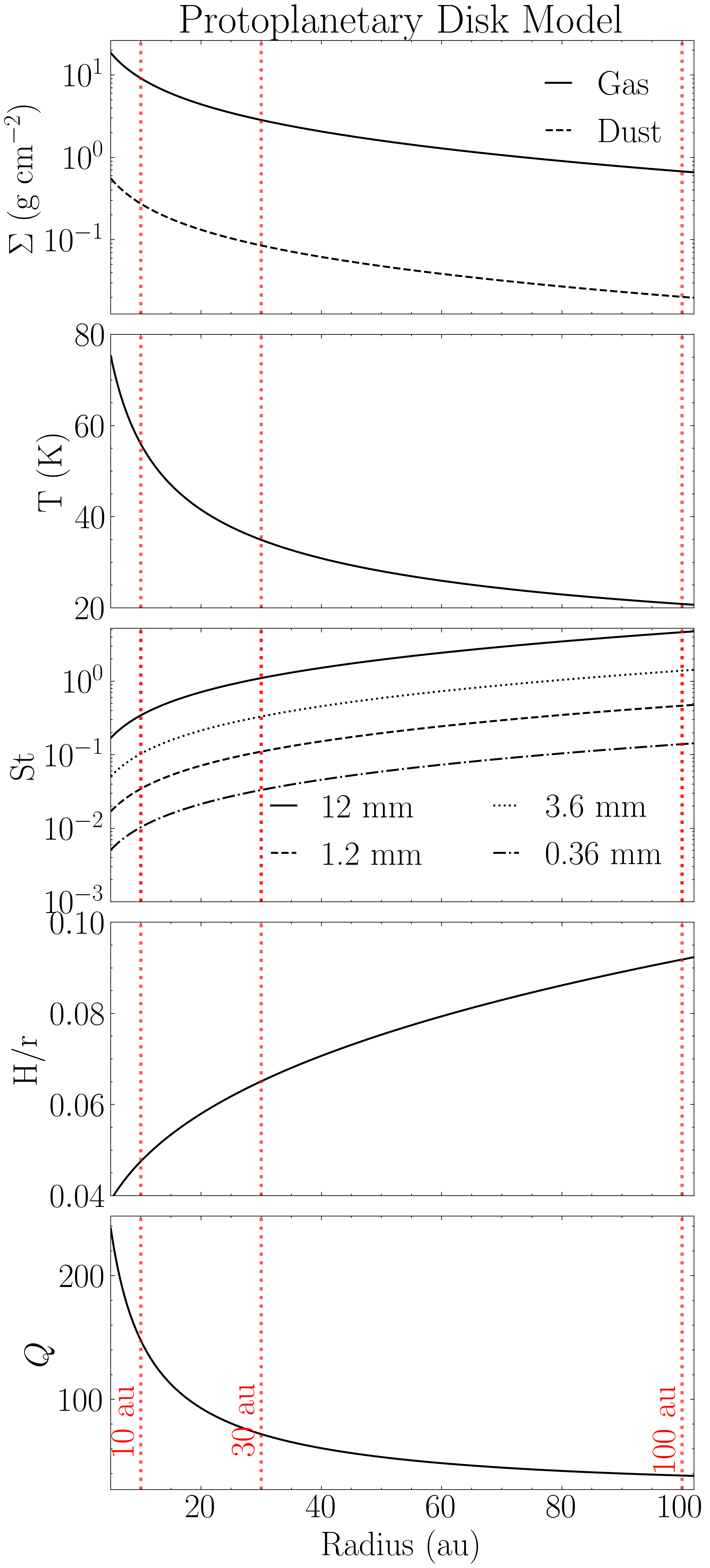
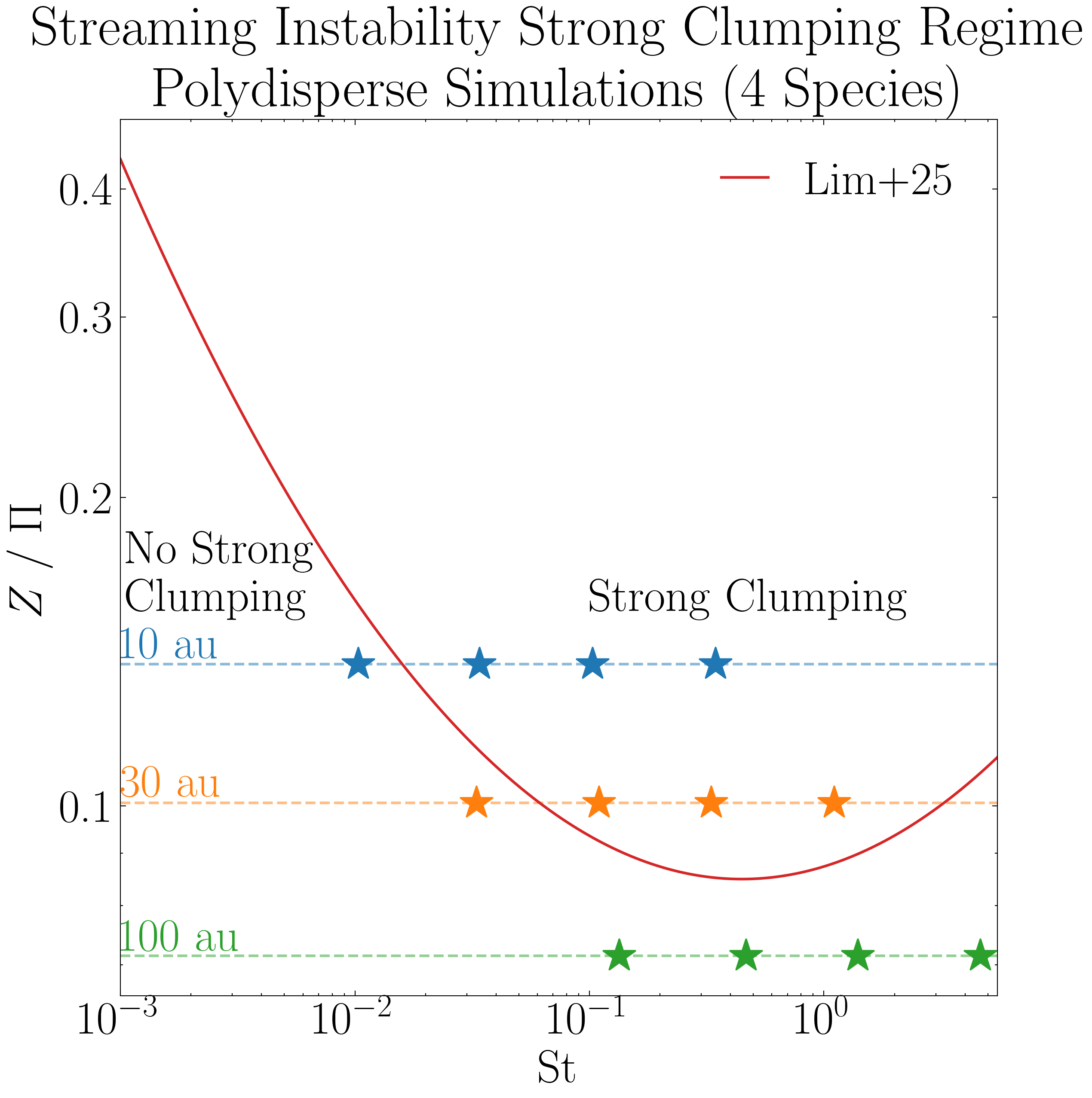
Figure 2 - SI Strong Clumping Regime
The following plot overlays the four species in our simulations, which evolve largely independently, on the strong clumping boundary for the streaming instability, as reported by Lim et al 2025.
import numpy as np
import matplotlib.pyplot as plt

try:
    import scienceplots
    plt.style.use('science')
    plt.rcParams.update({'font.size': 26,})
    plt.rcParams.update({'lines.linewidth': 1.5})
except:
    print('WARNING: Could not import scienceplots, please install via pip for proper figure formatting.')
    plt.style.use('default')


plt.figure(figsize=(8,8))

# Simulation parameters, stokes numbers and pressure gradient parameter
st10 = np.array([0.345, 0.103, 0.034, 0.0103])
st30 = np.array([1.105, 0.331, 0.110, 0.033])
st100 = np.array([4.651, 1.395, 0.465, 0.134])
Pi = np.array([0.0545, 0.0745, 0.105])

# The initial dust-to-gas ratio in our simulations (Equation 11)
Total_Z = 0.03

# In our simulations with four grain sizes and Z=0.03, the species act indepedent of one another (see Krapp et al. 2019)
Collective_Z = 0.03 / 4.

# The critical parameter adoped in this work (Z/Pi)
ratio_collective = Collective_Z / (Pi)

# Plot where the four species in each of the three simulations fall within this boundary
plt.scatter(st10, [ratio_collective[0]]*4, marker='*', facecolor='#1f77b4', s=350, edgecolor='#1f77b4')
plt.scatter(st30, [ratio_collective[1]]*4, marker='*', facecolor='#ff7f0e', s=350, edgecolor='#ff7f0e')
plt.scatter(st100, [ratio_collective[2]]*4, marker='*', facecolor='#2ca02c', s=350, edgecolor='#2ca02c')

# Adding horizontal dashed lines and text to denote where each simulation is in the disk
plt.axhline(y = ratio_collective[0], linestyle='--', color='#1f77b4', alpha=0.5)
plt.text(0.001, ratio_collective[0]+0.0017, "10 au", color='#1f77b4', fontweight="bold")

plt.axhline(y = ratio_collective[1], linestyle='--', color='#ff7f0e', alpha=0.5)
plt.text(0.001, ratio_collective[1]+0.0014, "30 au", color='#ff7f0e', fontweight="bold")

plt.axhline(y = ratio_collective[2], linestyle='--', color='#2ca02c', alpha=0.5)
plt.text(0.001, ratio_collective[2]+0.0008, "100 au", color='#2ca02c', fontweight="bold")

# Now plot the Li+25 boundary
# Stokes numbers to plot (x-axis)
x = np.arange(-3, 0.74037, 0.01)
St = 10 ** x

# Boundary parameters
Pi_ = 0.05
A = 0.10
B = 0.07
C = -2.36
C = C - np.log10(Pi_) # To show Z / Pi.

# Plot the critical boundary
Zcrit_array = (A * np.log10(St)**2) + (B * np.log10(St)) + C
Zcrit_array = 10 ** Zcrit_array
plt.loglog(St, Zcrit_array, color='#d62728', label="Lim+25")

# Label the clumping regions
plt.title('Streaming Instability Strong Clumping Regime\nPolydisperse Simulations (4 Species)')
plt.text(0.1, 0.155, "Strong Clumping", fontweight="bold")
plt.text(0.00105, 0.155, "No Strong\nClumping", fontweight="bold")
plt.xlabel("St"); plt.ylabel(r"$Z \ / \ \Pi$")
plt.yticks([0.1, 0.2, 0.3, 0.4], [str(y) for y in [0.1, 0.2, 0.3, 0.4]])
plt.xlim(1e-3, 5.5)

# Save
plt.legend(ncol=1, loc='upper right', handlelength=1)
plt.subplots_adjust(top=0.97, right=0.97, left=0.12, bottom=0.12)
plt.savefig('SI_criteria_Independent.png', dpi=300, bbox_inches='tight')
plt.show()
Radiative Transfer Analysis
The main analysis is shown below, during which all the relevant files are saved. These include the key results from the radiative transfer such as the mass excess and filling factor, as well as the 2D optical depth and corresponding intensity maps.
Simulation-based data is also saved, including the mass of the planetesimals as well as number of superparticles and the per-species maximum particle density over time.
This code was run 24 times – 4 ALMA bands x 3 disk locations x 2 opacity options (absorption only and absorption + scattering).
The saved data from this analysis has been made available for download here (2.4 GBs untarred). This is the path_to_save variable in the code below.
We have also made available for download the simulation data from the Pencil Code, which have been saved as .npy and .txt files to facilitate data-transfer. These files are needed for this analysis (the path_to_data variable below).
Download the simulation data here:
10 au simulation (5.11 GBs, 25 GBs untarred).
30 au simulation (6.02 GBs, 25 GBs untarred).
100 au simulation (7.61 GBs, 29 GBs untarred).
from protoRT import rtcube, disk_model
import astropy.constants as const
import matplotlib.pyplot as plt
import numpy as np


# The four ALMA wavelenghts (Bands 10, 7, 6, and 3)
alma_wavelengths_cm = [0.03, 0.087, 0.13, 0.3]

###
### THESE ARE THE THREE VARIABLES THAT ARE CHANGED! Observed Frequency (band index), Scattering Option (True/False), and Disk Location (10, 30, & 100) ###
###

# The index for the band that is being analyzed (indexes alma_wavelengths_cm list)
band = 0

# Whether to include scattering
include_scattering = True

# The location in the disk to be analyzed (10, 30 or 100 au)
r_ = 10

###
### Everything below is fixed
###

# The same disk model parameters from Fig. 1
# These are used to extract the corresponding disk params (sigma_g, T, & H) which are used to configure the cube for the radiative transfer
mass_disk = 0.02
M_star, M_disk = const.M_sun.cgs.value, mass_disk*const.M_sun.cgs.value
r, r_c = r_*const.au.cgs.value, 300*const.au.cgs.value
grain_rho = np.array([1.675, 1.675, 1.675, 1.675])
Z = 0.03
q = 3/7.
T0 = 150

# Define the disk model as the Sigma_g, T, and H are needed. NOTE: These parameters are independent of grain size/stokes number so no input needed
model = disk_model.Model(r, r_c, M_star, M_disk, Z=Z, q=q, T0=T0)

# The Stokes numbers used in the simulations which correspond to the disk model in Fig. 1
if r_ == 10:
        stoke = np.array([0.34454218, 0.10336265, 0.03445422, 0.01033627])
elif r_ == 30:
        stoke = np.array([1.10488383,0.33146515,0.11048838,0.03314651])
elif r_ == 100:
        stoke = np.array([4.65083295,1.39524989,0.4650833,0.13952499])
else:
        print('Invalid disk position! Options are: 10, 30, and 100')

# The paths to the Pencil Code data
save_dir = 'scattering' if include_scattering else 'absorption'
path_to_data = f'pencil_data_{r_}au/'

# Directory where analysis results will be saved
path_to_save = f'analysis/polydisperse/band{int(band+1)}/{save_dir}/{r_}au/'

# Normalization parameters used in the simulation set up
code_omega = 1
code_cs = 1
code_rho = 1

# Power law index for grain size distribution
p = 2.5

# Number of superparticles in the simulations
npar = 1000000

n_orbits = 101 # Number of snapshots saved

# The initial conditions are loaded and stored before the analysis begins
# This mass is used when computing the mass excess at all orbits as planetesimal formation removes available mass over time
init_var = np.load(path_to_data+'var_files/VAR0.npy')

# Empty lists to store quantities of interest, will be saved once all snapshots are analyzed
# These are the maximum particle densities (per scecies) which can be calculated from the
# density field that is made during the analysis. This density field (4D array) is too large to
# save for all orbits so this data is saved during analysis instead.  These are independent of the radiative transfer
max_rho_per_species = np.zeros((n_orbits, len(stoke))) # 101 Snapshots, 4 grain sizes

# Will also save the number of species in the domain over time (i.e., those not in sink particles)
num_particles = np.zeros((n_orbits, len(stoke)))

for var in np.arange(0, n_orbits, 1):
        print(f'Orbit {var} out of {n_orbits}')
        # Data cube (rhop) and z-axis (in units of H) from Pencil Code
        data_cube = np.load(path_to_data+'var_files/VAR'+str(var)+'.npy')
        axis = np.loadtxt(path_to_data+'axis.txt')
        #
        # Particle data from Pencil code
        aps = np.loadtxt(path_to_data+'aps_files/aps'+str(var)+'.txt')
        rhopswarm = np.loadtxt(path_to_data+'rhopswarm_files/rhopswarm'+str(var)+'.txt')
        particle_data = np.loadtxt(path_to_data+'ipars_positions_files/ipars_positions_'+str(var)+'.txt')
        ipars, species, positions_x, positions_y, positions_z = particle_data[:,0].astype(int), particle_data[:,1].astype(int), particle_data[:,2], particle_data[:,3], particle_data[:,4]
        #
        # Grid data from Pencil Code
        grid_data = np.loadtxt(path_to_data+'grid_xyz_polysg.txt')
        xgrid, ygrid, zgrid = grid_data[:,0], grid_data[:,1], grid_data[:,2]
        #
        # These are the attributes Pencil Code stores in read_param(), needed for our polydisperse analysis
        p2d_params = np.loadtxt(f'{path_to_data}/p2d_params_polysg.txt', dtype=str)
        #
        grid_func1, grid_func2, grid_func3 = p2d_params[0], p2d_params[1], p2d_params[2]
        particle_weight = float(p2d_params[3])
        mx, my, mz = int(p2d_params[4]), int(p2d_params[5]), int(p2d_params[6])
        nx, ny, nz = int(p2d_params[7]), int(p2d_params[8]), int(p2d_params[9])
        n1, n2, m1, m2, l1, l2 = int(p2d_params[10]), int(p2d_params[11]), int(p2d_params[12]), int(p2d_params[13]), int(p2d_params[14]), int(p2d_params[15])
        #
        # Run the main RT routine
        cube = rtcube.RadiativeTransferCube(
                data=data_cube,
                axis=axis,
                code_rho=code_rho,
                code_cs=code_cs,
                code_omega=code_omega,
                column_density=model.sigma_g,
                T=model.T,
                H=model.H,
                stoke=stoke,
                grain_rho=grain_rho,
                wavelength=alma_wavelengths_cm[band],
                include_scattering=include_scattering,
                kappa=None,
                sigma=None,
                p=p,
                npar=npar,
                ipars=ipars,
                xp=positions_x,
                yp=positions_y,
                zp=positions_z,
                xgrid=xgrid, # Same length as mx
                ygrid=ygrid, # Same length as my
                zgrid=zgrid, # Same length as mz
                rhopswarm=rhopswarm,
                particle_weight=particle_weight,
                grid_func=grid_func1, #Code assumes that grid_func1 = grid_func2 = grid_func3
                num_grid_points=mx, # Code assumes that mx = my = mz
                num_interp_points=nx, # Code assumes that nx = ny = nz
                index_limits_1=n1, # Code assumes that n1 = m1 = l1
                index_limits_2=n2, # Code assumes that n2 = m2 = l2
                aps=aps,
                eps_dtog=Z,
                init_var=init_var
                )
        #
        cube.configure()
        #
        # Save the key RT results and data parameters (mass excess, filling factor, unit density, cube mass, and mass for each present planetesimal)
        np.savetxt(path_to_save+f'cube_results_var_{var}.txt', np.r_[cube.mass_excess, cube.filling_factor, cube.unit_density, cube.mass, cube.proto_mass], header='Mass Excess | Filling Factor | Unit Density | Cube Mass | Planet Mass')
        #
        # Save the two-dimensional optical depth and intensity maps
        np.save(path_to_save+f'tau_intensity_{var}.npy', np.array([cube.tau, cube.intensity]))
        #
        # Only save the particle density data for the first run, as these are independent of the RT
        if band == 0 and scattering:
                # Calculate the max particle density per species
                for i in range(len(stoke)): max_rho_per_species[var, i] = np.max(cube.density_per_species[i])
                #
                # Convert the ipars array to numerical labels, first species is 1, second is 2, etc...
                _species_ = np.ceil(ipars / (npar / len(stoke)))
                for i in range(len(stoke)): num_particles[var, i] = len(np.where(_species_ == i+1)[0])

# Only need to save the particle density data for the first run, these are independent of the RT analysis
if band == 0 and scattering:
        # The particle evolution data is independent of the radiative transfer therefore will be saved on the main directory
        # Save the maximum particle densities over time, shown in first row of Fig. 3
        np.savetxt(path_to_save[:9]+f'max_densities_{r_}au.txt', max_rho_per_species)

        # Save the number of particles over time, shown in second row of Fig. 3
        np.savetxt(path_to_save[:9]+f'num_species_{r_}au.txt', num_particles)
Figure 3 - Simulations
The following code shows the time evolution of the three simulations. This uses the analysis results saved above and the time series dataframe provided in the simulation data.
import os
import re
import numpy as np
import matplotlib.pyplot as plt
from matplotlib.lines import Line2D
import pandas as pd
import astropy.constants as const

try:
    import scienceplots
    plt.style.use('science')
    plt.rcParams.update({'font.size': 32, 'lines.linewidth': 3.0})
except:
    print('WARNING: Could not import scienceplots, please install via pip for proper figure formatting.')
    plt.style.use('default')


# Function for loading the cube results in order (var 0 to 101)
def extract_number(fname):
    return int(re.search(r'\d+', fname).group())

# Function to extract the cube mass and planetesimal masses from the saved results
def load_mass_data(path):
    files = sorted([f for f in os.listdir(path) if 'cube_results' in f], key=extract_number)
    proto_mass, cube_mass = [], []
    for f in files:
        data = np.loadtxt(os.path.join(path, f))
        proto_mass.append(np.sum(data[4:]))
        cube_mass.append(data[3])
    return np.array(proto_mass), np.array(cube_mass)

# Function to load the time series dataframe (from the Pencil Code)
def load_time_series(filepath):
    columns = ['it', 't', 'dt', 'nparmax', 'ux2m', 'uy2m', 'uz2m', 'uxuym',
               'rhom', 'rhomin', 'rhomax', 'vpxm', 'xpm', 'xp2m', 'zpm', 'zp2m',
               'npmax', 'rhopm', 'rhopmax', 'nparsink', 'rhopinterp']
    df = pd.read_csv(filepath, delim_whitespace=True, names=columns, low_memory=False)
    return df['t'].values / (np.pi * 2), df['nparsink'].values

# We saved 101 snapshots, after each orbit
orbits = np.arange(0, 101, 1)

# Path to data, note that these are set assuming that the data and analysis folders are in the working directory

# Load the max particle densities per-species that was saved during analysis
max_density_10au = np.loadtxt('analysis/max_densities_10au.txt')
max_density_30au = np.loadtxt('analysis/max_densities_30au.txt')
max_density_100au = np.loadtxt('analysis/max_densities_100au.txt')

# Concat max particle density data into one array for convenience
max_density_data = np.c_[max_density_10au, max_density_30au, max_density_100au]

num_species10 = np.loadtxt('analysis/num_species_10au.txt')
num_species30 = np.loadtxt('analysis/num_species_30au.txt')
num_species100 = np.loadtxt('analysis/num_species_100au.txt')

# The mass in the simulation and that of the planetesimals is independent of the RT results, just use band1/scattering results here
proto_10, cube_10 = load_mass_data('analysis/polydisperse/band1/scattering/10au/')
proto_30, cube_30 = load_mass_data('analysis/polydisperse/band1/scattering/30au/')
proto_100, cube_100 = load_mass_data('analysis/polydisperse/band1/scattering/100au/')

# The time series data from simulations (Pencil Code)
ts_10, sink_10 = load_time_series('pencil_data_10au/time_series.dat')
ts_30, sink_30 = load_time_series('pencil_data_30au/time_series.dat')
ts_100, sink_100 = load_time_series('pencil_data_100au/time_series.dat')

# Max densities per location
maxes = np.split(max_density_data, 3, axis=1)
maxes_10, maxes_30, maxes_100 = [np.split(m, 4, axis=1) for m in maxes]

locations = {
    '10 au': {'maxes': maxes_10, 'roche': 1663.97, 'offset': 172, 'proto': proto_10, 'cube': cube_10, 'ts': ts_10, 'sink': sink_10, 'species': num_species10.T},
    '30 au': {'maxes': maxes_30, 'roche': 811.52, 'offset': 80, 'proto': proto_30, 'cube': cube_30, 'ts': ts_30, 'sink': sink_30, 'species': num_species30.T},
    '100 au': {'maxes': maxes_100, 'roche': 433.66, 'offset': 45, 'proto': proto_100, 'cube': cube_100, 'ts': ts_100, 'sink': sink_100, 'species': num_species100.T},
}

colors = ['#1f77b4', '#ff7f0e', '#2ca02c', '#d62728']
linestyles = ['-', '--', '-.', ':']
labels = ['1.2 cm', '0.36 cm', '0.12 cm', '0.036 cm']

# Plot
fig, axes = plt.subplots(4, 3, figsize=(24, 24), sharex='col')
plt.subplots_adjust(wspace=0.4)

for col, (loc, data) in enumerate(locations.items()):
    # Row 1: Max Density
    ax = axes[0, col]
    for i in range(4):
        ax.plot(orbits, data['maxes'][i], color=colors[i], linestyle=linestyles[i], alpha=0.7)
    ax.axhline(y=data['roche'], linestyle=(0, (1, 10)), linewidth=3.0, color='k')
    ax.text(41, data['roche'] + data['offset'], r'2$\rho_H$', color='k')
    ax.set_yscale('log')
    ax.set_xlim(0, 100)
    ax.set_ylim(8, 3000)
    if col == 0:
        ax.set_ylabel(r'$\rho_{d,\max} / \rho_{d,0}$')
    ax.set_title(loc)
    ax.tick_params(labelbottom=False)

    # Row 2: Particle Fractions
    ax = axes[1, col]
    for i in range(4):
        ax.plot(orbits, data['species'][i]/250000, color=colors[i], linestyle=linestyles[i], alpha=0.7)
    ax.set_ylim(0.15, 1.0073)
    if col == 0:
        ax.set_ylabel('Fraction of Superparticles')
    ax.tick_params(labelbottom=False)

    # Row 3: Number of Planetesimals
    ax = axes[2, col]
    ax.plot(data['ts'], data['sink'], color='k')
    ax.set_ylim(-0.09, 30)
    if col == 0:
        ax.set_ylabel(r'$\# \text{ of Planetesimals}$')
    ax.tick_params(labelbottom=False)

    # Row 4: Masses
    ax = axes[3, col]
    mass_Earth = data['proto'] / const.M_earth.cgs.value
    ax.plot(orbits, mass_Earth / 1e-6, color='k', linestyle='-')
    ax.set_xlim(0, 100)
    ax.set_ylim(bottom=0)
    ax.set_xlabel(r'$t / P$')
    if col == 0:
        ax.set_ylabel(r'Planetes. Mass ($10^{-6} M_{\oplus}$)')
    ax_twin = ax.twinx()
    dust_mass_frac = (data['cube'] - data['proto']) / (data['cube'][0] - data['proto'][0])
    ax_twin.plot(orbits, dust_mass_frac, color='k', linestyle='--')
    ax_twin.set_ylim(0.9875, 1.0001)
    if col == 2:
        ax_twin.set_ylabel('Fraction of Free Dust Mass')
        ax_twin.plot([], [], 'k-', label='Planetes. Mass')
        ax_twin.plot([], [], 'k--', label='Frac. of Dust Mass')
        ax_twin.legend(loc='center', handlelength=1.5, frameon=True, fancybox=True)

# Legend (grain sizes)
size_handles = [Line2D([0], [0], color=colors[i], linestyle=linestyles[i], label=label) for i, label in enumerate(labels)]
fig.legend(handles=size_handles, loc='upper center', title=r'$a$', frameon=True, fancybox=True, ncol=4, bbox_to_anchor=(0.5, 0.97))

fig.suptitle('Self-gravitating Streaming Instability Simulations', y=0.985)
plt.savefig('Simulation_Time_Evolution.png', dpi=300, bbox_inches='tight')
plt.show()
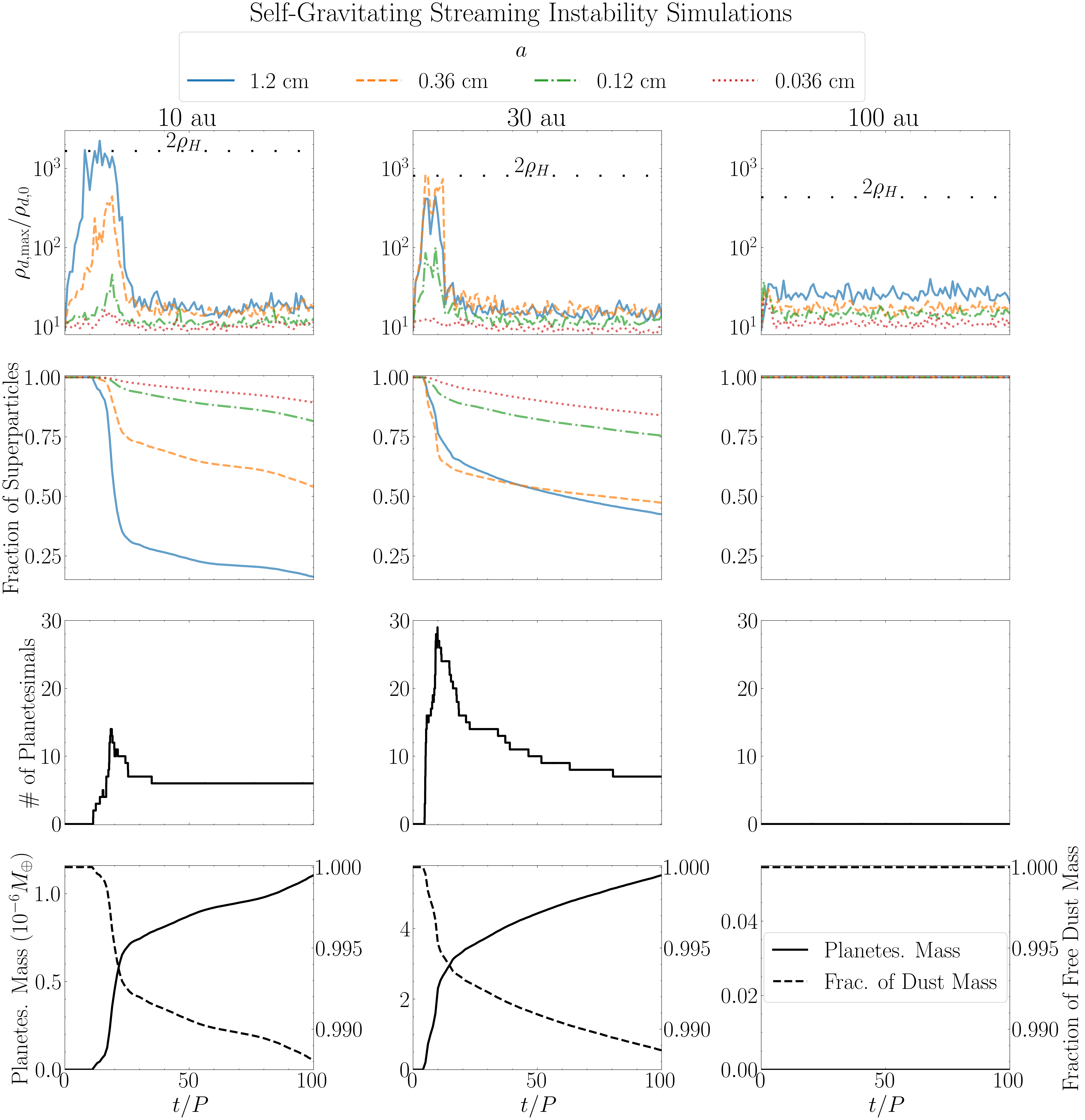
Figure 4 - Frequency-dependent Dust Opacities
This shows how we calculated the DSHARP opacities for the full grain size distribution, at the four ALMA bands used in the radiative transfer analysis. This was done using the compute_opacities module.
import numpy as np
import matplotlib.pyplot as plt
from matplotlib.lines import Line2D
from protoRT import compute_opacities

try:
    import scienceplots
    plt.style.use('science')
    plt.rcParams.update({'font.size': 32, 'lines.linewidth': 2.5})
except:
    print('WARNING: Could not import scienceplots, please install via pip for proper figure formatting.')
    plt.style.use('default')


# The four ALMA bands in our analysis and respective linestyle used
alma_wavelengths_cm = [0.03, 0.087, 0.13, 0.3]
linestyles = ['-', '--', '-.', ':']

# The full range of grain sizes from the DHSARP dust model
reference_grain = np.logspace(-5, 2, 200)

# Power-law index of grain size distribution
p = 2.5

# Full grain size distribution opacities
fig1, ax1 = plt.subplots(nrows=2, ncols=1, figsize=(10, 14), sharex=True)
fig1.suptitle('Size Averaged Opacities at ALMA Bands', y=1.03)

# Compute and Plot the Absorption & Scattering Opacities
for i, lam in enumerate(alma_wavelengths_cm):
    k_abs, k_sca, _ = compute_opacities.dsharp_model(p=p, wavelength=lam, grain_sizes=reference_grain, bin_approx=False)
    ax1[0].loglog(reference_grain, k_abs, linestyle=linestyles[i], color='blue')
    ax1[0].loglog(reference_grain, k_sca, linestyle=linestyles[i], color='red')

ax1[0].plot(1e-6, 0, color='blue', label=r'$\kappa_\nu$')
ax1[0].plot(1e-6, 0, color='red', label=r'$\sigma_\nu$')
ax1[0].set_ylabel(r'Dust Opacity ($\rm cm^2\,g^{-1}$)')
ax1[0].set_xlim(1e-3, 1e2)
ax1[0].set_ylim(1e-3, 200)
ax1[0].legend(loc='upper right', frameon=False, fancybox=True, handlelength=1.0)

# Corresponding Albedos
bands = [10, 7, 6, 3]
for i, lam in enumerate(alma_wavelengths_cm):
    k_abs, k_sca, _ = compute_opacities.dsharp_model(p=p, wavelength=lam, grain_sizes=reference_grain, bin_approx=False)
    albedo = k_sca / (k_abs + k_sca)
    ax1[1].plot(reference_grain, albedo, linestyle=linestyles[i], color='k')
    ax1[1].plot(1e-6, 0, linestyle=linestyles[i], color='k', label=f'{np.round(lam*10,3)} mm (Band {bands[i]})')

ax1[1].set_ylabel('Albedo')
ax1[1].set_xscale('log')
ax1[1].set_xlim(1e-3, 1e2)
ax1[1].set_ylim(0, 1)
ax1[1].set_xlabel(r'$a_{\rm max}$ (cm)')

lines, labels = ax1[1].get_legend_handles_labels()
fig1.legend(lines, labels, loc='upper center', ncol=2,
            frameon=True, fancybox=True, handlelength=0.8, bbox_to_anchor=(0.5, 1.005))

fig1.subplots_adjust(hspace=0.08)
fig1.savefig('full_dsharp_opacities.png', dpi=300, bbox_inches='tight')
plt.close(fig1)
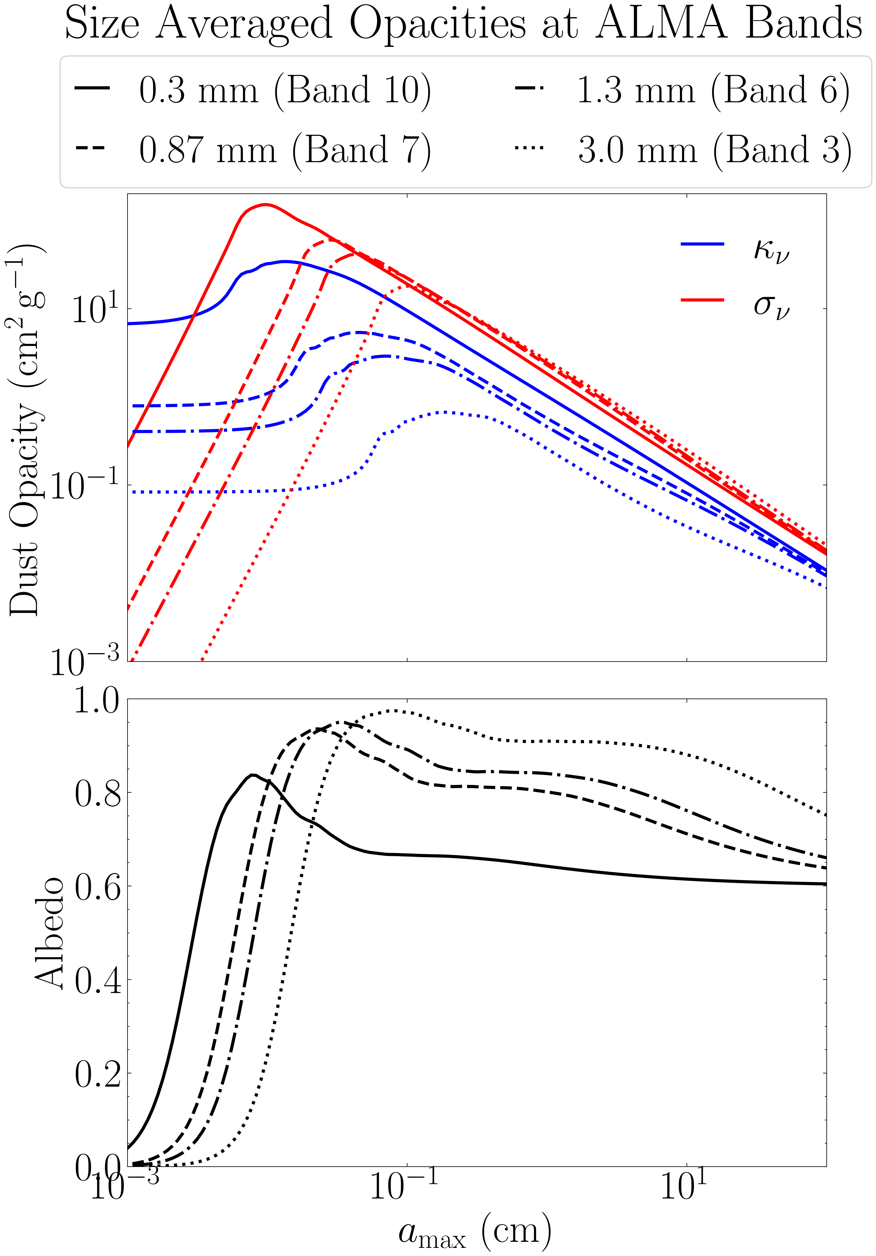
Figure 5 - Multi-Species Binned Opacities
The compute_opacities module also supports multi-species-based opacity calculations. In these cases, the grain size distributions must be binned according to the species. The size of each species corresponds to the maximum grain size in a single distribution, thus the minimum grain size must be set so as to avoid overlapping distributions. The code below shows these binned opacities for ALMA Band 7, and how they compare to that from the full grain size distribution. Using the full grain size distribution in multi-species models results in opacity overestimates, as the opacities from the smaller grains ends up contributing multiple times effectively overestimating the volume density of these smaller grains.
import numpy as np
import matplotlib.pyplot as plt
from matplotlib.lines import Line2D
from protoRT import compute_opacities

try:
    import scienceplots
    plt.style.use('science')
    plt.rcParams.update({'font.size': 32, 'lines.linewidth': 2.5})
except:
    print('WARNING: Could not import scienceplots, please install via pip for proper figure formatting.')
    plt.style.use('default')


# The four grain sizes in our simulations, used to bin the distributions
grain_sizes = [0.036, 0.12, 0.36, 1.2]

# The full range of grain sizes from the DHSARP dust model
reference_grain = np.logspace(-5, 2, 200)

# Power-law index of grain size distribution
p = 2.5

# Compute the binned and full opacities for 0.087 cm wavelength
opacity_abs_full, opacity_sca_full, _ = compute_opacities.dsharp_model(p=p, wavelength=0.087, grain_sizes=reference_grain, bin_approx=False)
opacity_abs_binned, opacity_sca_binned, bins = compute_opacities.dsharp_model(p=p, wavelength=0.087, grain_sizes=grain_sizes, bin_approx=True)

# Calculate the respective albedos
albedo_full = opacity_sca_full / (opacity_abs_full + opacity_sca_full)
albedo_binned = opacity_sca_binned / (opacity_abs_binned + opacity_sca_binned)

# Full vs Binned Opacities Plot
fig2, ax2 = plt.subplots(nrows=2, ncols=1, figsize=(10, 14), sharex=True)
fig2.suptitle('Polydisperse Binned Opacities', y=0.92)

ax2[0].loglog(reference_grain, opacity_abs_full, color='blue', linestyle='--')
ax2[0].loglog(reference_grain, opacity_sca_full, color='red', linestyle='--')
ax2[0].loglog(grain_sizes, opacity_abs_binned, color='blue', marker='^', linestyle='', markersize=12, alpha=0.7)
ax2[0].loglog(grain_sizes, opacity_sca_binned, color='red', marker='v', linestyle='', markersize=12, alpha=0.7)
ax2[0].set_ylabel(r'Dust Opacity ($\rm cm^2\,g^{-1}$)')
ax2[0].set_xlim(1e-3, 1e2)
ax2[0].set_ylim(1e-3, 1e2)

# Legends
ax2[0].add_artist(ax2[0].legend(
    handles=[Line2D([], [], color='blue', linestyle='--'),
             Line2D([], [], color='red', linestyle='--')],
    labels=[r'$\kappa_{\rm 0.87mm}$', r'$\sigma_{\rm 0.87mm}$'],
    title='Full', loc='upper right', frameon=True, fancybox=True, handlelength=0.7))
ax2[0].legend(
    handles=[Line2D([], [], color='blue', marker='^', linestyle='', markersize=12),
             Line2D([], [], color='red', marker='v', linestyle='', markersize=12)],
    labels=[r'$\kappa_{\rm 0.87mm}$', r'$\sigma_{\rm 0.87mm}$'],
    title='Binned', loc='lower right', frameon=True, fancybox=True, handlelength=0.7)

# Green bin guides
ax2[0].vlines(1.02e-5, 1.2e-3, 0.24, color='green', linestyle=(0, (1, 1)))
for i, gsize in enumerate(grain_sizes):
    ax2[0].loglog(bins[i], [1.2e-3]*len(bins[i]), color='green', linestyle=(0, (1, 1)))
    ax2[0].vlines(gsize, 1.2e-3, 0.24, color='green', linestyle=(0, (1, 1)))
    ax2[0].text(gsize * 0.95, 1.2e-3 * 1.3, rf'$a_{{\max}}={gsize}\,$cm', rotation=90, ha='right', color='green', size=32)

# Plot corresponding Albedos
ax2[1].plot(reference_grain, albedo_full, color='k', linestyle='--', label=r'$\omega_{\rm 0.87mm}$ (Full)')
ax2[1].plot(grain_sizes, albedo_binned, color=(0.5, 0, 0.5), marker='D', linestyle='', markersize=12, alpha=0.7, label=r'$\omega_{\rm 0.87mm}$ (Binned)')
ax2[1].set_xlabel(r'$a_{\rm max}$ (cm)')
ax2[1].set_ylabel('Albedo')
ax2[1].set_xscale('log')
ax2[1].set_xlim(1e-3, 1e2)
ax2[1].set_ylim(0, 1)
ax2[1].legend(loc='center right', frameon=True, fancybox=True, handlelength=0.7)

cc1, cc2 = 0.005, 0.3 # To place the green bins
ax2[1].vlines(1.02e-5, cc1, cc2, color='green', linestyle=(0, (1, 1)))
for i, gsize in enumerate(grain_sizes):
    ax2[1].plot(bins[i], [cc1]*len(bins[i]), color='green', linestyle=(0, (1, 1)))
    ax2[1].vlines(gsize, cc1, cc2, color='green', linestyle=(0, (1, 1)))
    ax2[1].text(gsize * 0.95, cc1 * 5.22, f'Bin {i+1}', rotation=90, ha='right', color='green', size=32)

fig2.subplots_adjust(hspace=0.08)
fig2.savefig('binned_opacities_example.png', dpi=300, bbox_inches='tight')
plt.close(fig2)
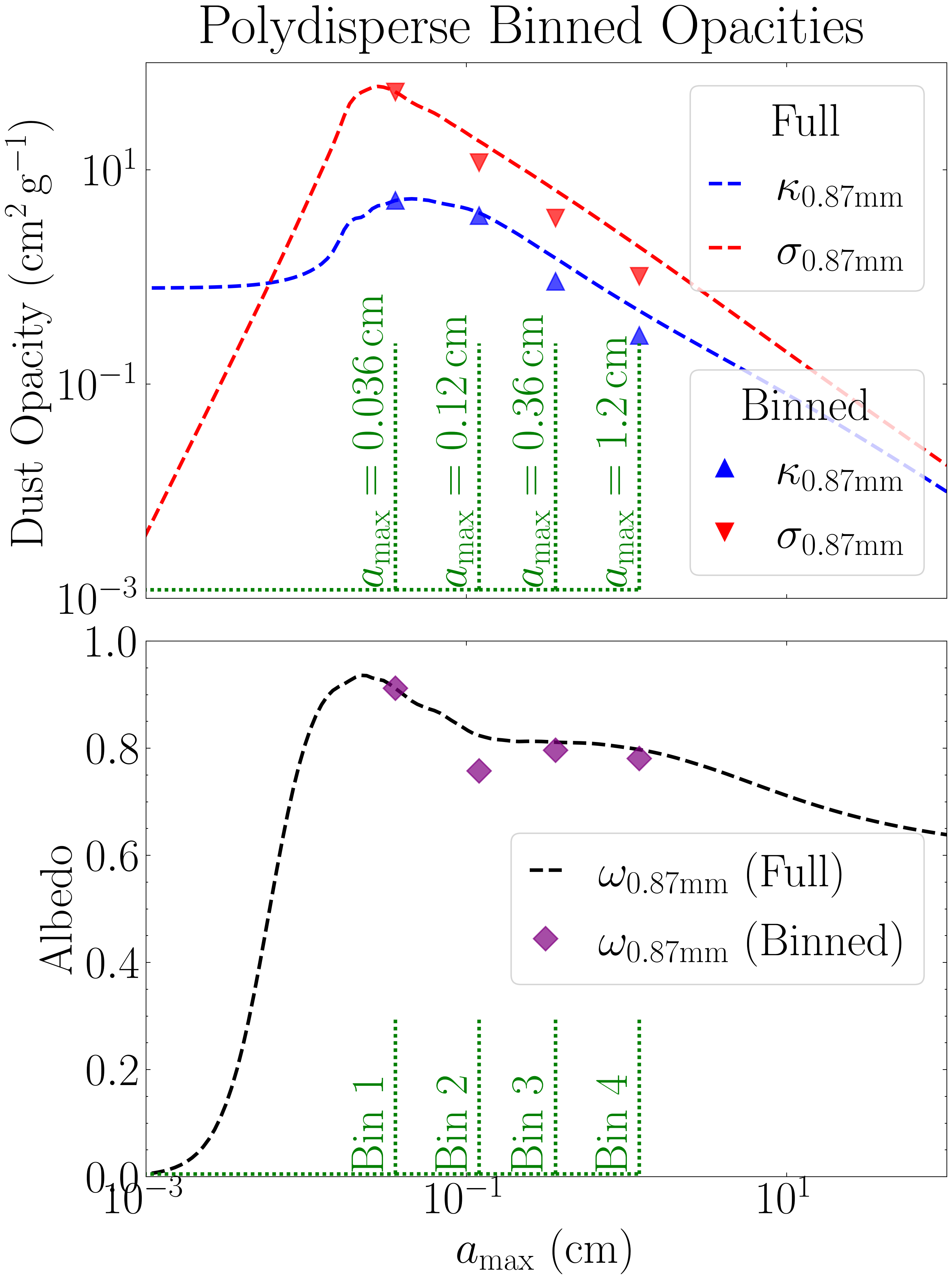
Figure 6 - Time Evolution of Dust Distribution
The figure below shows the vertically and azimuthally averaged dust density as a function of time for all three simulations. A red dashed line marks the time of peak dust density, corresponding to the moment when streaming instability-driven clumping produces significant overdensities. At this point, the dust density exceeds the background level by factors of 9.46, 5.68, and 1.75 for the simulations at 10, 30, and 100 au, respectively.
import os
import re
import numpy as np
import matplotlib.pyplot as plt
from mpl_toolkits.axes_grid1 import make_axes_locatable

try:
    import scienceplots
    plt.style.use('science')
    plt.rcParams.update({'font.size': 32, 'lines.linewidth': 2.5})
except:
    print('WARNING: Could not import scienceplots, please install via pip for proper figure formatting.')
    plt.style.use('default')


def extract_number(fname):
    """Return the first integer that appears in *fname* (used for natural sort)."""
    return int(re.search(r'\d+', fname).group())

def load_rhopmx(path):
    """
    Load polydisperse self-gravity simulation (either 10, 30, or 100 au run), and
    compute the azimuthally averaged density as a function of (x, t).

    Parameters
    ----------
    path : The path to the var_files data folder of the particular simulation

    Returns
    -------
    rhopmx : np.ndarray
        2-D array with shape (time, x)
    t_peak : int
        time index at which the global maximum occurs
    """

    fnames = sorted([f for f in os.listdir(path) if f.endswith('.npy')], key=extract_number)

    averaged = np.zeros((len(fnames), 256))
    for i, fname in enumerate(fnames):
        data = np.load(os.path.join(path, fname)) # The rhop datacube -- shape = (y, z, x)
        averaged[i] = data.mean(axis=(0, 1)) # x-profile (mean over y & z)

    rhopmx = averaged # (time, x)
    t_peak = np.argmax(rhopmx.max(axis=1)) # index of global maximum
    return rhopmx, t_peak

# Load data for 10 au, 30 au, and 100 au runs, note that the path below assumpes the data folder is in the working directory
rhopmx_list, t_peaks = zip(*(load_rhopmx(f'pencil_data_{i}au/var_files/') for i in (10, 30, 100)))
titles = ['10 au', '30 au', '100 au']
time = np.arange(rhopmx_list[0].shape[0]) # assumes equal length


# Plot
fig, axs = plt.subplots(1, 3, figsize=(24, 8))

# Shared colour scale
vmin = min(np.log10(r).min() for r in rhopmx_list)
vmax = max(np.log10(r).max() for r in rhopmx_list)
levels = np.linspace(vmin, vmax, 256)

for j, (rho, t_peak) in enumerate(zip(rhopmx_list, t_peaks)):
    cf = axs[j].contourf(
        time, np.linspace(-0.1, 0.1, 256),
        np.log10(rho).T, levels=levels, cmap='viridis', extend='both'
    )
    axs[j].set_title(titles[j])
    axs[j].set_xlabel(r'$t / P$')
    axs[j].set_xticks([0, 20, 40, 60, 80, 100])
    axs[j].set_yticks([-0.1, -0.05, 0, 0.05, 0.1])
    axs[j].axvline(t_peak, color='red', ls='--', alpha=0.6, label=r'$\rho_{d,\mathrm{max}} / \rho_{d,0}$')
    axs[j].legend(loc='upper right', frameon=True, fancybox=True, handlelength=0.5)
    axs[j].set_aspect('auto')

# Left-most y-axis label
axs[0].set_ylabel(r'$x / H$')
for ax in axs[1:]:
    ax.tick_params(labelleft=False)

# Shared colorbar beside the last axis
divider = make_axes_locatable(axs[-1])
cax = divider.append_axes("right", size="5%", pad=0.4)
cb = fig.colorbar(cf, cax=cax)
cb.set_label(r'$\log_{10}\!\left(\rho_{d} / \rho_{d,0}\right)$')

fig.savefig('poly_max_density.png', dpi=300, bbox_inches='tight')
plt.show()
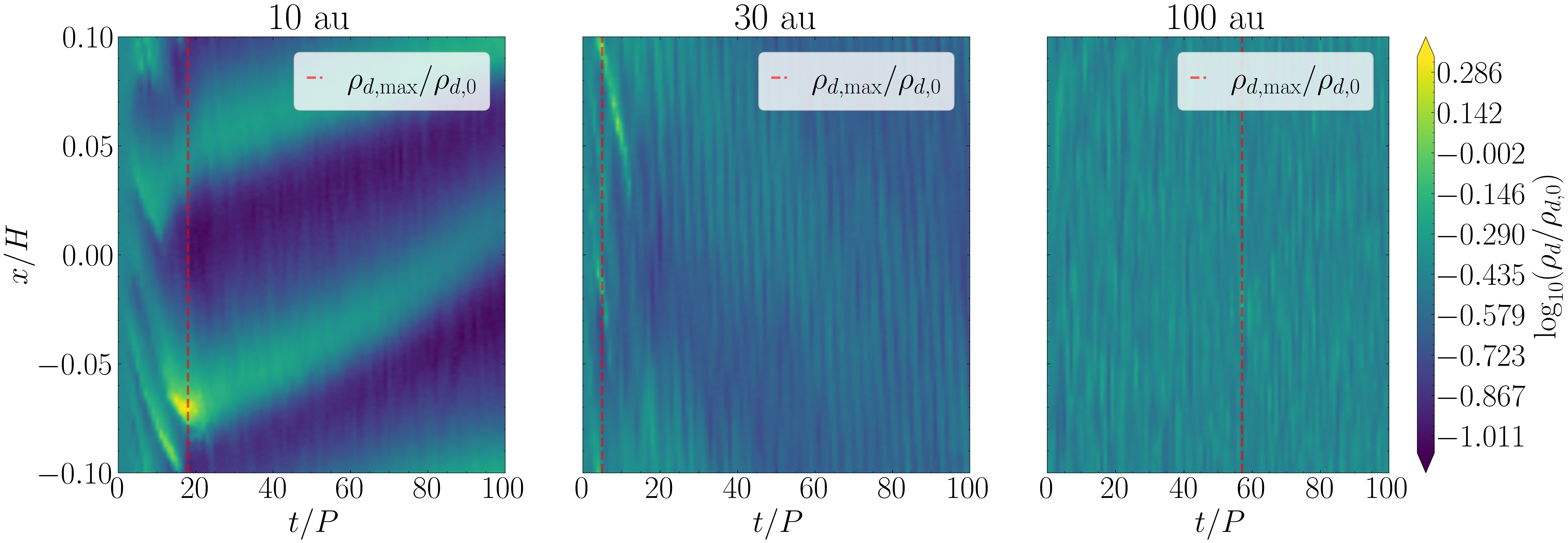
Figure 7 - Optical Depth and Intensity Maps
The effective optical depth and corresponding intensity maps at the output plane are displayed below. This example shows only the results at one particular orbit (the time of maximum density as denoted in Fig. 6), and at ALMA Band 7 (0.87 mm). The key metrics are annotated in red, including the mean optical depth and the corresponding filling factor, as well as the optically thick fraction and the mass excess.
from StreamingInstability_YJ14 import shearing_box, disk_model
import astropy.constants as const
import numpy as np
import matplotlib.pyplot as plt
import os, re
from matplotlib import gridspec
from mpl_toolkits.axes_grid1 import make_axes_locatable

try:
    import scienceplots
    plt.style.use('science')
    plt.rcParams.update({'font.size': 32, 'lines.linewidth': 2.5})
except:
    print('WARNING: Could not import scienceplots, please install via pip for proper figure formatting.')
    plt.style.use('default')

def return_bnu(r, wave):
    """Planck function at radius r (cm) and wavelength wave (cm).

    Parameters
    ----------
    r : The radius of the disk at which to compute the intensity, in cm.
    wave : The observational wavelength, in cm.

    Returns
    -------
    b_nu : float
        The intensity of an ideal blackbody at the temperature of the given disk locationm
    """

    # The disk model we adopt in this work
    mass_disk = 0.02
    M_star, M_disk = const.M_sun.cgs.value, mass_disk * const.M_sun.cgs.value
    r_c = 300 * const.au.cgs.value

    # Define the disk model to calculate the temperature
    model = disk_model.Model(r, r_c, M_star, M_disk, Z=0.03, q=3/7., T0=150)

    # Convert wavelength to frequency (Hz)
    freq = const.c.cgs.value / wave

    # The intensity of an ideal blackbody at that temperature
    B_nu = 2 * const.h.cgs.value * freq**3 / (const.c.cgs.value**2 * (np.exp(const.h.cgs.value * freq / (const.k_B.cgs.value * model.T)) - 1))

    return B_nu

def extract_number(fname):
    """ Helper function for loading the var files in order (*_var_*.npy) """
    return int(re.search(r'\d+', fname).group())

def load_rhopmx(path):
    """ Helpfer function to load the var files and compute the maximum dust density observer at each orbit """
    fnames = sorted([f for f in os.listdir(path) if f.endswith('.npy')], key=extract_number)
    averaged = np.zeros((256, len(fnames)))
    for i, f in enumerate(fnames):
        averaged[:, i] = np.mean(np.load(os.path.join(path, f)), axis=(0, 1))
    return np.transpose(averaged)

# Load the var files and compute the maximum dust density for each simulation (note that the data directories are assumed to be in the working directory)
rhopmx1 = load_rhopmx('pencil_data_10au/var_files/')
rhopmx2 = load_rhopmx('pencil_data_30au/var_files/')
rhopmx3 = load_rhopmx('pencil_data_100au/var_files/')

# Ran simulation for 100 orbits
time = np.arange(0, 101, 1)

# indices of peak frame for each run (needed for cube_results_var_*.txt)
ind1 = np.where(rhopmx1 == np.max(rhopmx1))[0]
ind2 = np.where(rhopmx2 == np.max(rhopmx2))[0]
ind3 = np.where(rhopmx3 == np.max(rhopmx3))[0]

# Load the radiative transfer results (effective optical depth and intensity maps)
specific_alma_wavelength = 0.087 # Observational wavelength in cm, this figure only considers ALMA Band 7

# Load the optical depth and intensity maps, note that ALMA Band 7 data is saved as band2 in the data directory
# Note that the analysis directory is assumed to be in the current working directory
base_path = 'analysis/polydisperse/band2/scattering/'
tau_int1 = np.load(f'{base_path}/10au/tau_intensity_{ind1[0]}.npy')
tau_int2 = np.load(f'{base_path}/30au/tau_intensity_{ind2[0]}.npy')
tau_int3 = np.load(f'{base_path}/100au/tau_intensity_{ind3[0]}.npy')

data = np.loadtxt(f'{base_path}/10au/cube_results_var_{ind1[0]}.txt')
me0 = data[0]
ff0 = data[1]

data = np.loadtxt(f'{base_path}/30au/cube_results_var_{ind2[0]}.txt')
me1 = data[0]
ff1 = data[1]

data = np.loadtxt(f'{base_path}/100au/cube_results_var_{ind3[0]}.txt')
me2 = data[0]
ff2 = data[1]


# Plot
fig2 = plt.figure(figsize=(26, 16))
gs = gridspec.GridSpec(2, 4, width_ratios=[1, 1, 1, 0.05], wspace=0.05, hspace=0.05)
axs = np.empty((2, 3), dtype=object)

# Effective optical depth maps
vmin_m = min(np.log10(t[0]).min() for t in [tau_int1, tau_int2, tau_int3])
vmax_m = max(np.log10(t[0]).max() for t in [tau_int1, tau_int2, tau_int3])
levels_m = np.linspace(vmin_m, vmax_m, 256)

for j, ti in enumerate([tau_int1, tau_int2, tau_int3]):
    ax = fig2.add_subplot(gs[0, j]); axs[0, j] = ax
    cf_m = ax.contourf(np.linspace(-0.1, 0.1, 256), np.linspace(-0.1, 0.1, 256),
                       np.log10(ti[0]), levels=levels_m, cmap='plasma', extend='both')
    ax.set_xlim(-0.1, 0.1)
    ax.set_xticks([-0.1, -0.05, 0, 0.05, 0.1])
    ax.set_yticks([-0.1, -0.05, 0, 0.05, 0.1])
    ax.set_xticklabels(['-0.1', '-0.05', '0.0', '0.05', '0.1'])
    ax.set_yticklabels(['-0.1', '-0.05', '0.0', '0.05', '0.1'])
    ax.tick_params(labelbottom=False)
    ax.set_aspect('equal')
    ax.set_ylabel(r'$y/H$') if j == 0 else ax.tick_params(labelleft=False)
    ax.set_title(['10 au', '30 au', '100 au'][j])
    # The annotations we show in red
    mean_m = [np.mean(tau_int1[0]), np.mean(tau_int2[0]), np.mean(tau_int3[0])]
    ff = [ff0, ff1, ff2]
    txt = (r"$\begin{array}{c}"
           rf"\langle \tau_{{0.87\,\mathrm{{mm}}}}^{{\mathrm{{eff}}}}\rangle={mean_m[j]:.1f}\\"
           rf"f_{{\rm fill}}={ff[j]:.2f}"
           r"\end{array}$")
    ax.text(0.5, 0.13, txt, transform=ax.transAxes, ha='center', va='center',
            color='red', bbox=dict(boxstyle='round,pad=0.5', facecolor='white',
                                   edgecolor='red', linewidth=2, alpha=0.6))

# colorbar for above optical depth map
cax_top = fig2.add_subplot(gs[0, 3])
fig2.colorbar(cf_m, cax=cax_top).set_label(
    r'$\log_{10}\!\left(\tau_{0.87\mathrm{mm}}^{\mathrm{eff}}\right)$')

# Intensity maps
vmin_b = min(np.log10(t[1]).min() for t in [tau_int1, tau_int2, tau_int3])
vmax_b = max(np.log10(t[1]).max() for t in [tau_int1, tau_int2, tau_int3])
levels_b = np.linspace(vmin_b, vmax_b, 256)

for j, ti in enumerate([tau_int1, tau_int2, tau_int3]):
    ax = fig2.add_subplot(gs[1, j]); axs[1, j] = ax
    cf_b = ax.contourf(np.linspace(-0.1, 0.1, 256), np.linspace(-0.1, 0.1, 256),
                       np.log10(ti[1]), levels=levels_b, cmap='coolwarm',
                       extend='both')
    ax.set_xlim(-0.1, 0.1)
    ax.set_xticks([-0.1, -0.05, 0, 0.05, 0.1])
    ax.set_yticks([-0.1, -0.05, 0, 0.05, 0.1])
    ax.set_xticklabels(['-0.1', '-0.05', '0.0', '0.05', '0.1'])
    ax.set_yticklabels(['-0.1', '-0.05', '0.0', '0.05', '0.1'])
    ax.set_xlabel(r'$x/H$'); ax.set_aspect('equal')
    ax.set_ylabel(r'$y/H$') if j == 0 else ax.tick_params(labelleft=False)
    # The annotations we show in red
    me = [me0, me1, me2]
    # Optically thick fraction: mean(intensity)/Planckian
    mean_b = [np.mean(tau_int1[1]) / return_bnu(10*const.au.cgs.value, specific_alma_wavelength),
              np.mean(tau_int2[1]) / return_bnu(30*const.au.cgs.value, specific_alma_wavelength),
              np.mean(tau_int3[1]) / return_bnu(100*const.au.cgs.value, specific_alma_wavelength)]
    txt = (r"$\begin{array}{c}"
           rf"f_{{\rm thick}}={mean_b[j]:.2f}\\"
           rf"\Lambda={me[j]:.1f}"
           r"\end{array}$")
    ax.text(0.5, 0.13, txt, transform=ax.transAxes, ha='center', va='center',
            color='red', bbox=dict(boxstyle='round,pad=0.5', facecolor='white',
                                   edgecolor='red', linewidth=2, alpha=0.6))

# colorbar for above intensity map
cax_bot = fig2.add_subplot(gs[1, 3])
fig2.colorbar(cf_b, cax=cax_bot).set_label(
    r'$\log_{10}\!\left(I_{0.87\,\mathrm{mm}}\right)$' +
    '\n(erg s$^{-1}$ cm$^{-2}$ Hz$^{-1}$ sr$^{-1}$)')

fig2.savefig('RT_results_ALMA_Band_7.png', dpi=300, bbox_inches='tight')
plt.show()
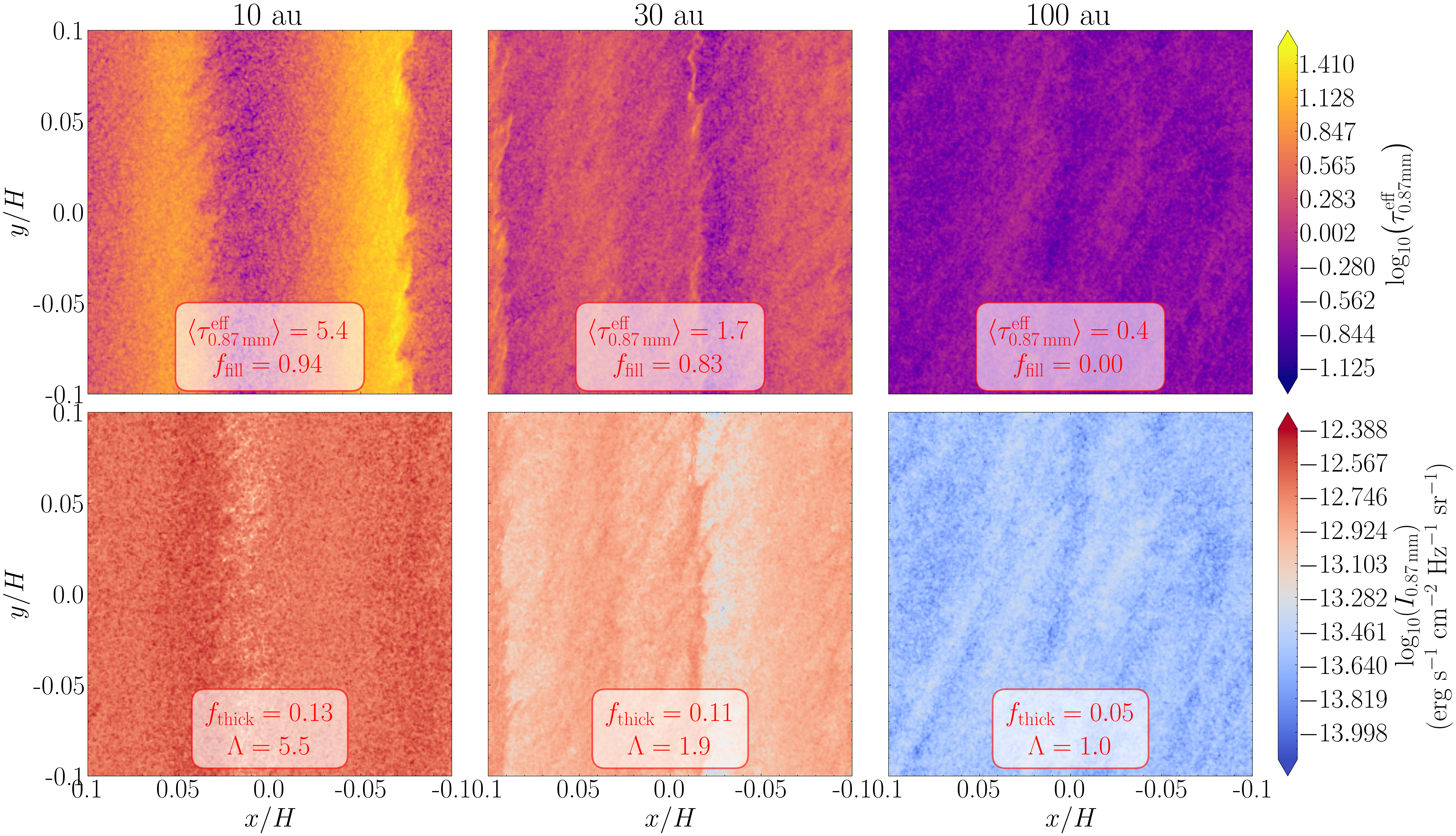
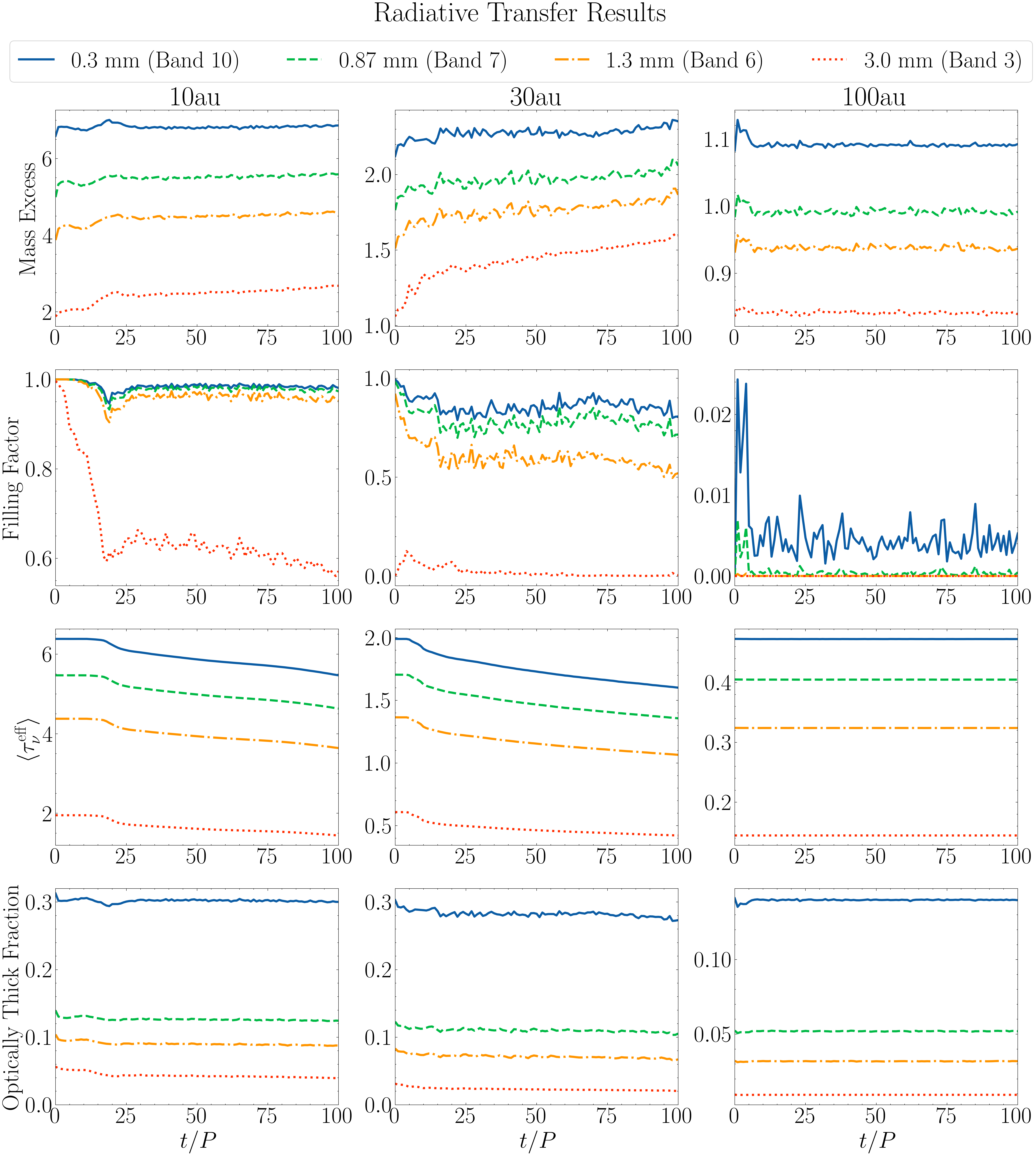
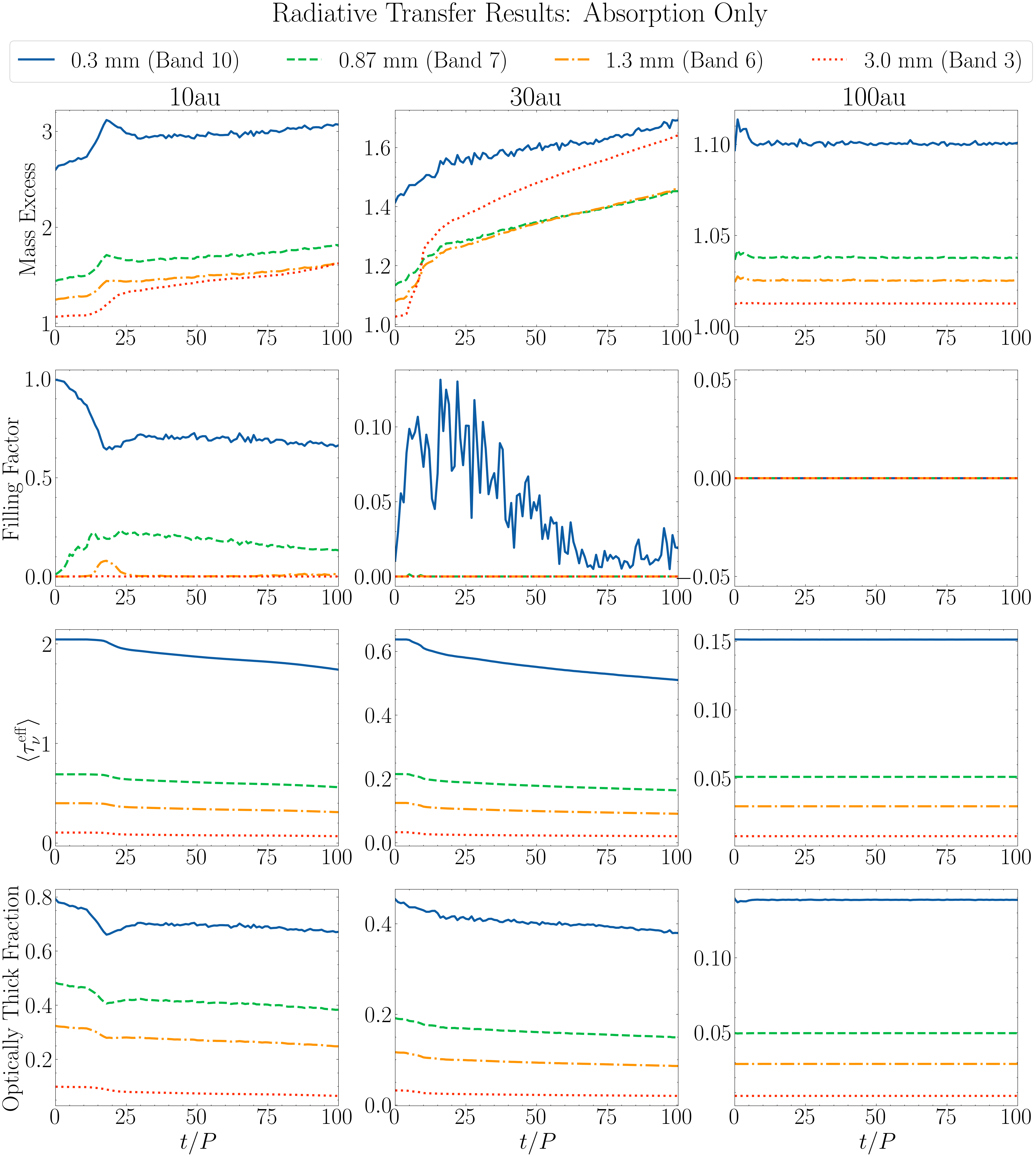
Figure 8 & 9 - Radiative Transfer Results
These are the main results from our analysis, showing how the key parameters (mass excess, filling factor, mean optical depth, and corresponding optically thick fractions) evolve over time. These are presented column-wise, with the 10 au results on the left, the 30 au in the middle, and the 100 au results on the right.
This plotting procedure includes an include_scattering variable, which if set to True will show the results when the scattering opacities are considered in the radiative transfer. If set to False, the absorption-only scenario is shown. This uses the data files available in the analysis directory that was saved.
import os
import numpy as np
import matplotlib.pyplot as plt
import astropy.constants as const
from StreamingInstability_YJ14 import shearing_box, disk_model

try:
    import scienceplots
    plt.style.use('science')
    plt.rcParams.update({'font.size': 32, 'lines.linewidth': 3.0})
except:
    print('WARNING: Could not import scienceplots, please install via pip for proper figure formatting.')
    plt.style.use('default')


def return_bnu(r, wave):
    """Planck function at radius r (cm) and wavelength wave (cm).

    Parameters
    ----------
    r : The radius of the disk at which to compute the intensity, in cm.
    wave : The observational wavelength, in cm.

    Returns
    -------
    b_nu : float
        The intensity of an ideal blackbody at the temperature of the given disk locationm
    """

    # The disk model we adopt in this work
    mass_disk = 0.02
    M_star, M_disk = const.M_sun.cgs.value, mass_disk * const.M_sun.cgs.value
    r_c = 300 * const.au.cgs.value

    # Define the disk model to calculate the temperature
    model = disk_model.Model(r, r_c, M_star, M_disk, Z=0.03, q=3/7., T0=150)

    # Convert wavelength to frequency (Hz)
    freq = const.c.cgs.value / wave

    # The intensity of an ideal blackbody at that temperature
    B_nu = 2 * const.h.cgs.value * freq**3 / (const.c.cgs.value**2 * (np.exp(const.h.cgs.value * freq / (const.k_B.cgs.value * model.T)) - 1))

    return B_nu


# The four ALMA Bands we analyzed
alma_wavelengths_cm = [0.03, 0.087, 0.13, 0.3]

# The name of the directories where the ALMA Band-specific data is saved (corresponds to the alma_wavelenghts_cm list above)
bands = ['band1', 'band2', 'band3', 'band4']

# The three locations of our simulations
locations = ['10au', '30au', '100au']

# The path to the analysis directory, assuming it is in the current working directory
base_path = 'analysis/polydisperse/' #'/Users/daniel/Desktop/SI_Project/final_mass_excess/polydisperse'

# Whether to consider the scattering opacities in the radiative transfer
include_scattering = True

# The directory to use depending on whether scattering is enabled
specific_directory = 'scattering' if include_scattering else 'absorption'

# Empty dictionary to store all relevant metrics
data = {}
for location in locations:
    data[location] = {}
    for band in bands:
        data[location][band] = {
            'orbits': [],
            'mass_excess': [],
            'filling_factor': [],
            'optically_thick_frac': [],
            'mean_taus': []
        }

for location in locations:
    for band in bands:
        # Empty lists to store the data
        orbits = []
        mass_excess_list = []
        filling_factor_list = []
        optically_thick_frac_list = []
        mean_taus_list = []
        #
        path = os.path.join(base_path, band, specific_directory, location)
        #
        for orbit in range(101):
            try:
                cube_results_file = os.path.join(path, f'cube_results_var_{orbit}.txt')
                cube_results = np.loadtxt(cube_results_file)
                mass_excess = cube_results[0]
                filling_factor = cube_results[1]
                #
                tau_intensity_file = os.path.join(path, f'tau_intensity_{orbit}.npy')
                tau_intensity = np.load(tau_intensity_file)
                #
                intensity_map = tau_intensity[1] # The intensity map is the second axis in the array
                #
                # The location, corresponds to the name of the directories as they are saved in the analysis folder
                if location == '10au':
                    r_ = 10*const.au.cgs.value
                elif location == '30au':
                    r_ = 30*const.au.cgs.value
                elif location == '100au':
                    r_ = 100*const.au.cgs.value

                if band == 'band1':
                    wave_ = alma_wavelengths_cm[0]
                if band == 'band2':
                    wave_ = alma_wavelengths_cm[1]
                if band == 'band3':
                    wave_ = alma_wavelengths_cm[2]
                if band == 'band4':
                    wave_ = alma_wavelengths_cm[3]

                # Compute the optically thick fraction
                f_thick = np.mean(intensity_map) / return_bnu(r_, wave_)
                #
                orbits.append(orbit)
                mass_excess_list.append(mass_excess)
                filling_factor_list.append(filling_factor)
                optically_thick_frac_list.append(f_thick)
                mean_taus_list.append(np.mean(tau_intensity[0]))
                #
            except Exception as e:
                print(f"Error loading data for {location} {band} orbit {orbit}: {e}")
                break
        #
        data[location][band]['orbits'] = orbits
        data[location][band]['mass_excess'] = mass_excess_list
        data[location][band]['filling_factor'] = filling_factor_list
        data[location][band]['optically_thick_frac'] = optically_thick_frac_list
        data[location][band]['mean_taus'] = mean_taus_list


# For plotting labeling and formatting
location_to_col = {'10au': 0, '30au': 1, '100au': 2} # First column is 10 au, second is 30, third is 100
bands_cm = [0.03, 0.087, 0.13, 0.3] # For labeling
ALMA_bands = [10, 7, 6, 3] # For labeling
linestyles = ['-', '--', '-.', ':'] # Corresponding linestyles
band_linestyles = dict(zip(bands, linestyles))

# Plot
fig, axes = plt.subplots(4, 3, figsize=(24, 26), sharex='col')
plt.subplots_adjust(top=0.85)

counter = 0 # To control indexing of the formatting lists/labels defined above
for location in locations:
    col = location_to_col[location]
    for counter, band in enumerate(bands):
        linestyle = band_linestyles[band]
        # Extract the data
        orbits = data[location][band]['orbits']
        mass_excess = data[location][band]['mass_excess']
        filling_factor = data[location][band]['filling_factor']
        f_thick = data[location][band]['optically_thick_frac']
        mean_taus = data[location][band]['mean_taus']

        # mass excess
        label = f'{np.array(bands_cm)[counter]*10:.2f} mm (Band {ALMA_bands[counter]})' if counter == 1 else \
                f'{np.array(bands_cm)[counter]*10:.1f} mm (Band {ALMA_bands[counter]})'
        axes[0][col].plot(orbits, mass_excess, linestyle=linestyle, label=label)

        # filling factor
        axes[1][col].plot(orbits, filling_factor, linestyle=linestyle)
        # optically thick fraction
        axes[3][col].plot(orbits, f_thick, linestyle=linestyle)
        # mean taus
        axes[2][col].plot(orbits, mean_taus, linestyle=linestyle)

# Set the axes limits
axes[0][2].set_ylim(1) if specific_directory == 'absorption' else None
axes[3][0].set_ylim((0.0, 0.32)) if specific_directory == 'scattering' else None
axes[3][1].set_ylim((0.0, 0.32)) if specific_directory == 'scattering' else None

# Set titles for the columns
for col, location in enumerate(locations): axes[0][col].set_title(location.replace('au', ' au'))

# Set the axes labels
axes[0][0].set_ylabel('Mass Excess')
axes[1][0].set_ylabel('Filling Factor')
axes[3][0].set_ylabel('Optically Thick Fraction')
axes[2][0].set_ylabel(r'$\langle \tau_\nu^{\rm eff} \rangle$')

# Set xlabels for the bottom row only
for col in range(3): axes[3][col].set_xlabel(r'$t / P$')

# Set xlim for all subplots
for row in range(4):
    for col in range(3):
        axes[row][col].set_xlim(0, 100)

# Set tick params for all subplots
for row in range(4):
    for col in range(3):
        axes[row][col].tick_params(labelbottom=True, labelleft=True)

# Get handles and labels for legend from the first subplot
handles, labels = axes[0][0].get_legend_handles_labels()

# Place the legend below the suptitle
fig.legend(handles, labels, loc='upper center', frameon=True, fancybox=True, handlelength=1.5, ncol=4, bbox_to_anchor=(0.5, 0.91))

# Add suptitle
if specific_directory == 'scattering':
    fig.suptitle('Radiative Transfer Results', y=0.93)
    plt.savefig(f'results_{specific_directory}.png', dpi=300, bbox_inches='tight')
else:
    fig.suptitle('Radiative Transfer Results: Absorption-only', y=0.93)
    plt.savefig(f'results_{specific_directory}.png', dpi=300, bbox_inches='tight')

plt.show()